Evolution on Fitness landscapes
contributed by Bhaskar Kumawat
How DNA works
The simplest case of evolution in nature is encountered in organisms like bacteria. Bacterial cells are biological machines that produce and use proteins to metabolize resources in their environment, and subsequently reproduce to create copies of themselves. The production of these proteins is delegated to a triad of processes that form the “central dogma” of molecular biology. The first level of this cascade is a polymeric molecule called DNA, which is sometimes referred to as the building block of life. Through a series of steps, the sequences of components comprising this molecule is converted into a protein that then performs the functions necessary to sustain life in the cell.
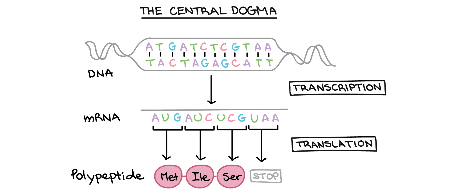
In the first process, called transcription, the DNA strand is copied into a RNA strand (another polymeric molecule like DNA). Subsequently, this RNA strand is “translated” into a protein by molecular assemblies called ribosomes. In this process, the ribosome reads three nucleic acids at once (collectively called a codon), and adds an amino acid to a growing protein chain. The completed protein chains fold together to create the final protein that then participates in cellular reactions like metabolism and reproduction.
DNA replication and the genotype
Most of the chemical complexity of a DNA molecule can be ignored by assuming it to be a combination of four monomeric units called the nucleic acids—Adenine (A), Thymine (T), Glutamine (G), and Cytosine (C). In a bacterial cell, these nucleic acids form a circular “strand” of DNA called its genome. The exact sequence of nucleic acids that form the genome is called the genotype. Replication of the genome during cellular reproduction proceeds in a way that is distinct from the creation of proteins. When a cell reproduces, a molecule called a DNA polymerase reads the DNA genome to create a copy of it, that is then transferred to the daughter cell. However, the copying is not generally perfect and can create errors or “mutations” in the chromosome. These mutations in turn, affect the production of proteins and their functionality in the cell.

Genotype spaces
A single DNA sequence in the bacterial genome can thus mutate in various ways to create different combinations of nucleic acids in the daughter cells. All possible mutated versions of genotypes thus form a genotype space in which these variants of the genome lie. An example of a simple genotype space created from only two nucleotides is given below.
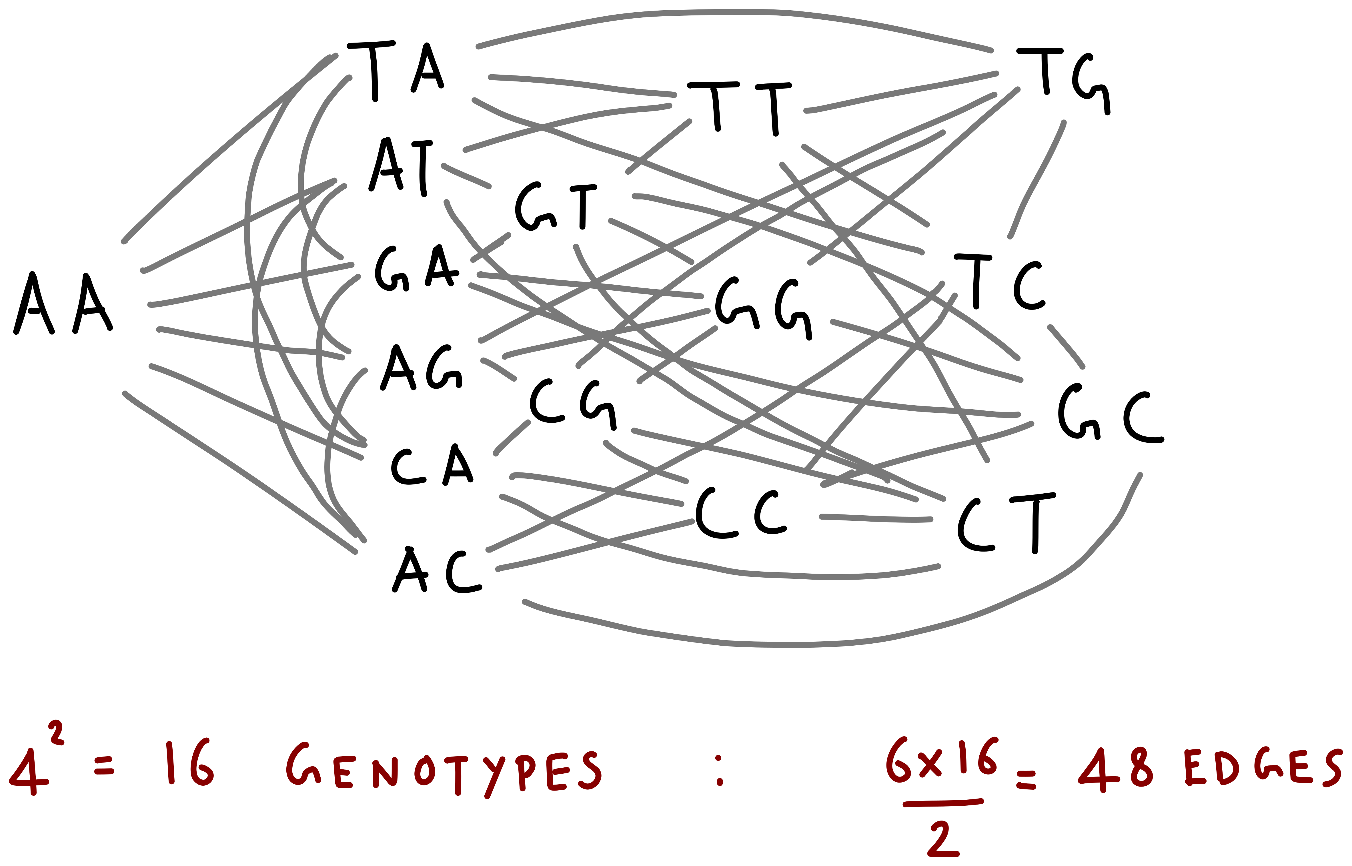
There are two interesting things to note here. First, the genotype space looks somewhat like a network, with genotype sequences as the nodes and edges connecting sequences that are mutants of each other. Second, even for 2 nucleotides, there are a total of \(4^2= 16\) genotypes in this space. Bacterial genomes, or even individual genes are much longer, with a usual gene being around 100 nucelotides long. The genotype space of such a gene thus forms a immensely large space of \(4^{100}\) genotypes. Visualizing and working with such large spaces for the purpose of our demonstration is difficult. Instead, we abstract away the network details and consider a nicer, linear genotypes space. In this space, mutations only happen between adjacent genotypes.

Fitness landscapes
Each mutation can have different effects on the phenotype (i.e., the traits) of a newly created cell. For example, a mutation that affects the folding of an important metabolic protein can reduce the fitness of the organism. On the other hand, mutations can sometimes create surprising enhancements to fitness by allowing new or more efficient biochemical pathways to emerge. These mutations can also be neutral, having no effect on the fitness of the resulting organism (in fact, it is widely believed that most mutations that occur in biological organisms are neutral).
More concretely, fitness can be measured on an absolute scale where it is simply the rate of doubling of a cell when grown in isolation. Assuming we have a way to measure this fitness for every possible genotype, we can assign each node in the genotype space a fitness-value. This creates a fitness landscape that overlays the genotype space and over which populations evolve. Theoretical biologists generally use different models to approximate fitness landscapes. Additive landscapes, NK model, and the royal staircase landscape are some examples of these on a realistic high-dimensional genotype space.
On a one-dimensional genotype space however, we have very few options. In terms of complexity, there are essentially four different flavors of a fitness landscape determined by the correlation between adjacent fitness values.

How evolution works
The fitness landscape captures how organisms can change their strategy to survive in their. However, that is not the complete picture. A population is a group of organisms (and hence of genotypes) that exist in the same space and evolve on this landscape. The way these populations evolve is not always straightforward. For example, in the conventional “survival of the fitness” narrative, all members of a population should simply mutate to the fittest genotype on the landscape and stay there. However, both real fitness landscapes and the process of evolution is significantly more complex than this adage reveals.
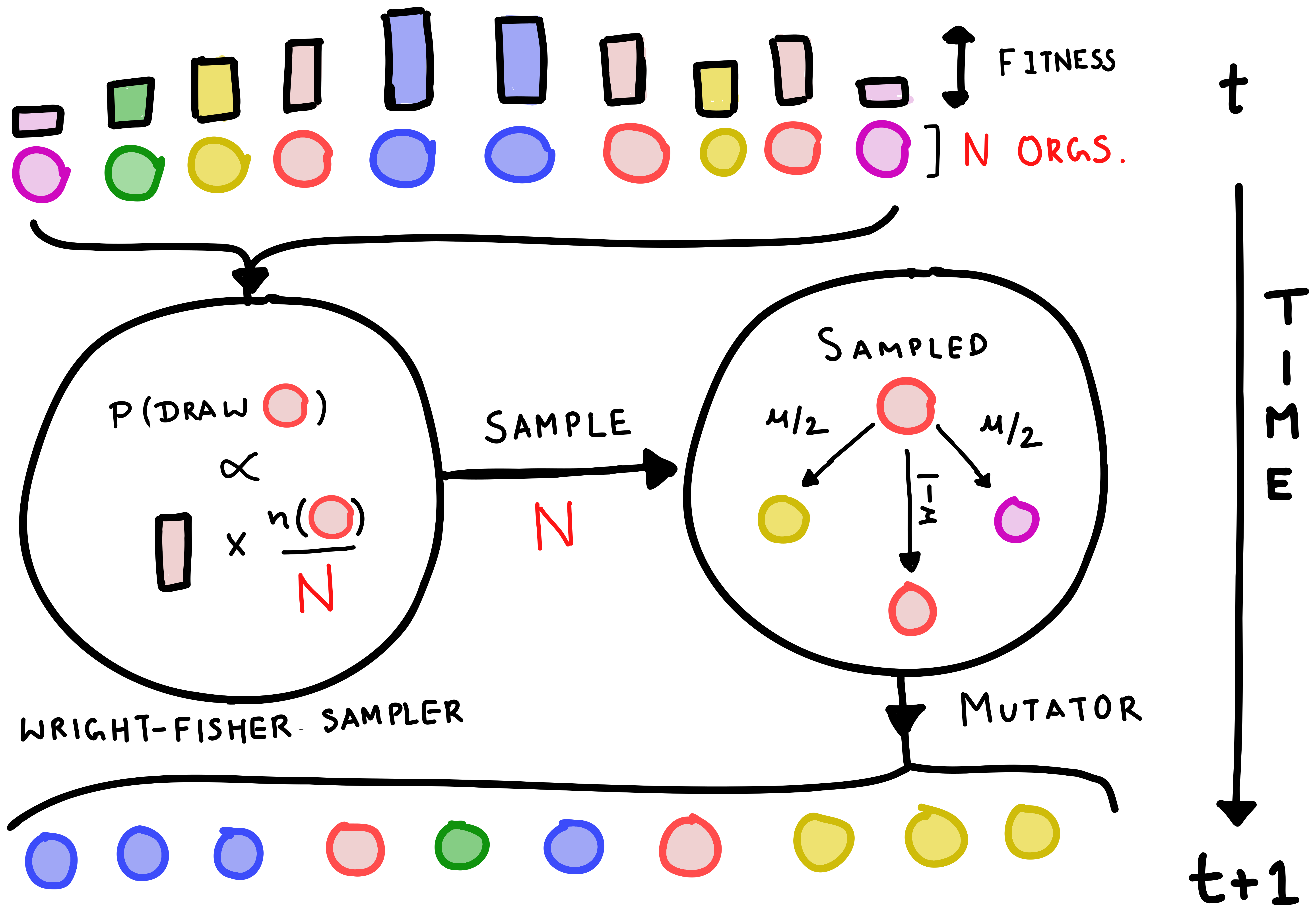
The Wright-Fisher model is a simple algorithmic approach to evolution that attempts to capture some of this complexity. In this model, the population size is fixed and time passes in discrete steps or generations. Every generation, the genotypes present in the population are resampled with replacement—with a probability proportional to their fitness and frequency in the current generation—to reconstitute a new population with the same number of organisms. Mutations can be added to the model by changing the genotype with a small probability (\(\mu\)) which stands for the mutation rate during replication.
Two genotypes
The following simulation models the Wright-Fisher process for a two-genotype space (called A and B) with a finite population size and mutation rate. Try modifying the sliders to see how the population reacts to a change in the relative fitness of B to A, the population size, and the mutation rate.
Even in this simple simulation, some interesting things can be noted about the nature of the evolutionary process. For example,
- Small populations have much stronger demographic noise compared to large populations (i.e., when we lower the population size, the fluctuations in population fractions are much larger).
- If the population size is large enough (to reduce demographic noise), increasing the relative fitness of B increases the fraction of population that has the B genotype. This difference is amplified if you decrease the mutation rate.
- Even when the fitnesses of B and A are exactly equal, one of the genotypes can achieve fixation (i.e. becomes the only genotype in the population, this phenomena is generally referred to as genetic drift). This is especially true when the population size is small and mutation rate is low.
Many genotypes
The model can be easily extended to a multiple genotypes. The following simulation models \(k\) different genotypes with fitness values drawn from a normal distribution with finite variance. The translucent red bars show the relative fitness values while the blue bars denote the fraction of organisms having a particular genotype.
Under certain conditions, the populations in this model shows an interesting behavior sometimes called a “wandering phenomenon”. This occurs when the mutation rate, the population sizes, and the fitness differences between genotypes are relatively small such that the spread of the population in the space is much smaller than the number of genotypes. In this case, the distribution of genotypes forms a finite cluster and moves arbitrarily in the space. (For example, try \(N=200\), \(\mu=0.0316\), \(k=50\) and a zero fitness variance).
Fitness seascapes
The ecological settings in which life exists are not as stagnant as a single fitness landscape conveys. For example, a bacterial cell may have to face both freezing temperatures and extreme warmth as the seasons change (or even during a day). Thus, a fitness landscape that changes with time is a more appropriate model for changing environments. A set of such interconnected fitness landscapes that switch between each other is sometimes called a fitness seascape.
Like landscapes, fitness seascapes also come in different flavors, with the two most common ones being a moving fitness optimum and a strong-tradeoff seascape.
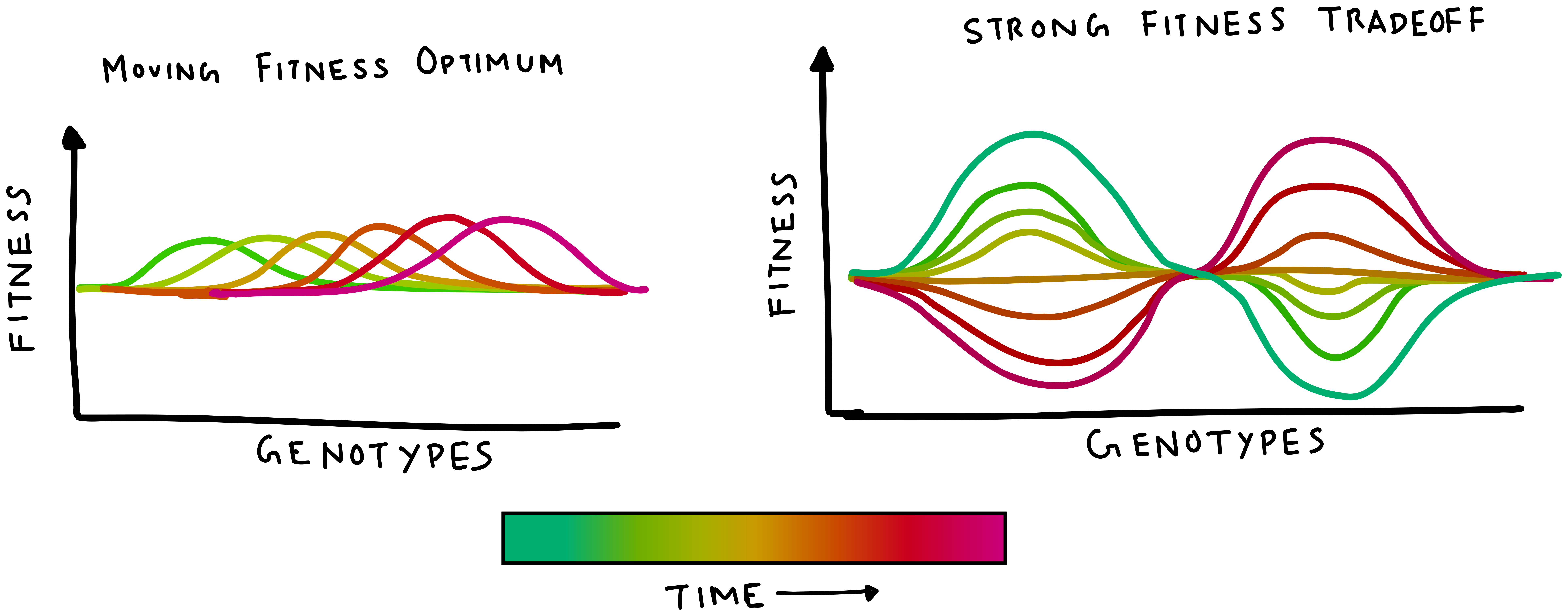
The following simulation presents a 200-genotype space with either the moving optimum or tradeoff seascape, and with a finite population evolving on it. The sliders can be adjusted to simulate a faster or slower rate of environment change.
[### Seascapes applet]
From fitness to phenotype
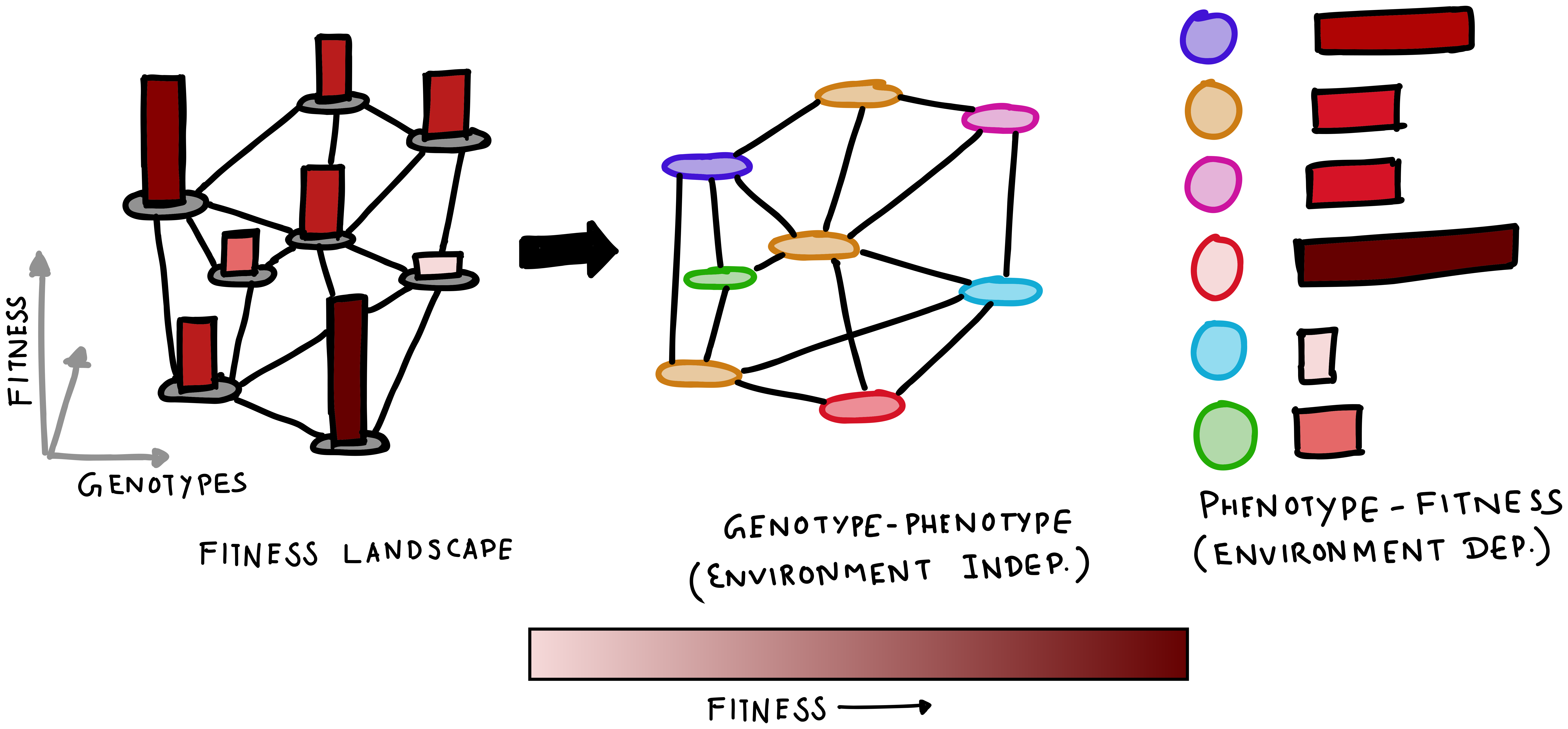
Keeping track of how fitness changes across environments can be difficult. However, under certain permissive conditions, the phenotype of the organism (i.e., the set of traits it has) is the major determinant of how fit it is going to be in an environment. For example, whether or not a cell can produce a heat-shock protein determines its ability to survive in a hot environment. Thus, when discussing dynamic fitness landscapes, it is usually easier to assign fitness values through a genotype-phenotype map. The fitness landscape, which is essentially a genotype-fitness mapping can then be decomposed into a genotype-phenotype and phenotype-fitness mapping.
The primary advantage of this decomposition lies in the fact that the genotype-phenotype variant is generally invariant across environments, and a change in external conditions only changes how the phenotype translates to the rate of growth. Additionally, because the genotype-phenotype map is redundant (with multiple genotype having the same phenotype), it requires a far fewer number of fitness values to be measured. The following example shows an example of fitness landscapes that is decomposed this way.
A hint of evolvability
Evolvability is the idea that certain populations can be differentially reactive to changing selective pressures. Thus, the term can be used to capture a population’s capacity for adaptation. Whether the evolutionary process can enhance a population’s evolvability has been the topic of a great debate in the field of evolutionary biology. In recent work, we have shown that this enhancement does occur under certain environments and through multiple pathways. One of these pathways works via the localization of populations on phenotypic boundaries in the genotype space when the environment changes. This localization can be observed in the seascape simulation as well, but the results are slightly more striking in two dimensions.
The following simulation presents a two-dimensional genotype space on which a population can be seen evolving. Here, each pixel is a genotype and mutations only occur between adjacent genotypes. White squares are genotypes with no organisms, and the intensity of the color represents the concentration of organisms on a particular genotype. The sliders can be used to modify the population size, mutation rate, and speed of the simulation. Additionally, the user can drag their mouse around the space to draw what is referred to as a neutral network. A neutral network is a set of genotypes that have the same phenotype (and thus the same fitness). The relative fitness slider can be used to adjust the ratio of fitness of the neutral network genotypes to the rest of the genotype space.
As one can expect, drawing a neutral network with a high fitness immediately makes the population find and localize in this high fitness area of the genotype space. Further, using the time-average button will show you that most organisms in these neutral networks reside in the center of the network, far from the edges where mutations that decrease fitness are possible. This idea is sometimes referred to as mutational robustness.
On the other hand, something interesting happens when the environment is allowed to switch to a state where the neutral network genotypes now have a smaller fitness (which can be triggered by increasing the environment switching probability). Time averaging the population in this switching environment reveals an elevated fraction of organisms with genotypes on the boundary of the neutral network, where it interfaces with genotypes of a different phenotype. Thus, the environmental switching induces an interesting steady state where the population prefers parts of the genotype space where phenotype switching mutations are more likely. A changing environment can thus promote the evolution of evolvability in these populations!